The following examples include the data that can be copied/paste directly into the X-Y Data box on the main page.
Example 1. Hydraulics
Example 2. Water Quality Modeling
Example 3. Cost Estimate
Many water quality models express the hydraulic characteristics (velocity, depth) for rivers and streams in terms of flow (Q) in cubic feet per second (CFS) using discharge coefficients, which are simple power functions. These power functions were generally found to fit observed data such that:
Velocity = aQb, Depth = cQd
The United States Geological Survey (USGS) maintains an inventory current and historical stream gages for the nation. Some gages provide real-time stream flow information collected every 15 minutes, daily average flows, highest instantaneous peak flow for a given year, miscellaneous flow measurements, or a combination of all of these. Of interest to this example are the miscellaneous flow measurements, which are made by hand and are used to develop rating curves for automated stream monitoring equipment or to provide some flow information for a site. Miscellaneous flow measurements will often include Area, Width, Velocity at a location.
In the this example, we are going to calculate discharge coefficients for velocity and depth at stream gage USGS 04256059, Black River at Dadville NY located near the Village of Lowville, NY, by linear regression using the method of Ordinary Least Squares (OLS) and the power transformation y = axb. Average stream depth for a given measurement was estimated by dividing area by width (Area/Width). Below are delimited x-y pairs for flow versus velocity and flow versus depth that can be copied/pasted for the analysis.
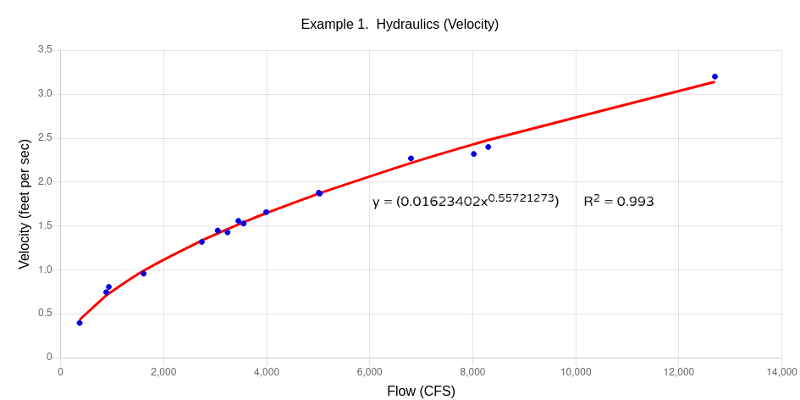
Results of the regression analysis for velocity result in discharge coefficients a = 0.01623, b = 0.5572. The coefficient of determination (R2) was 0.993, indicating a very good fit. The resulting equation v = 0.01623Q0.5572 can be used to estimate the stream velocity at a specific flow.
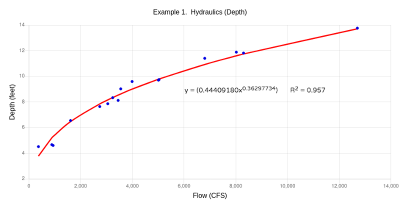
Results of the regression analysis for depth result in discharge coefficients c = 0.44409, d = 0.36298. The coefficient of determination (R2) was 0.957, also indicating a very good fit. The resulting equation d = 0.44409Q0.36298 can be used to estimate the stream depth at a specific flow.
Being a wise engineer, you can can now estimate the hydraulic characteristics for a flow of 500 CFS to be used in a water quality model. The calculated velocity is 0.01623*5000.5572 = 0.52 feet/sec. The calculated depth is 0.44409*5000.36298 = 4.24 feet.


| Date |
|---|
| 09/14/2020 |
| 05/18/2020 |
| 11/05/2019 |
| 10/09/2019 |
| 06/13/2019 |
| 04/01/2019 |
| 11/26/2018 |
| 08/06/2018 |
| 06/14/2018 |
| 04/12/2018 |
| 04/12/2018 |
| 04/09/2018 |
| 11/06/2017 |
| 10/17/2017 |
| 09/08/2017 |
| 04/06/2017 |
| Flow (cfs) | Velocity (feet/sec) |
|---|---|
| 368 | 0.4 |
| 2740 | 1.32 |
| 8300 | 2.4 |
| 5010 | 1.88 |
| 3550 | 1.53 |
| 6800 | 2.27 |
| 3990 | 1.66 |
| 936 | 0.81 |
| 885 | 0.75 |
| 3450 | 1.56 |
| 3240 | 1.43 |
| 5030 | 1.87 |
| 8020 | 2.32 |
| 1610 | 0.96 |
| 3050 | 1.45 |
| 12700 | 3.2 |
| Flow (cfs) | Depth (feet) |
|---|---|
| 368 | 4.53 |
| 2740 | 7.65 |
| 8300 | 11.82 |
| 5010 | 9.71 |
| 3550 | 9.03 |
| 6800 | 11.41 |
| 3990 | 9.60 |
| 936 | 4.62 |
| 885 | 4.68 |
| 3450 | 8.13 |
| 3240 | 8.34 |
| 5030 | 9.75 |
| 8020 | 11.89 |
| 1610 | 6.56 |
| 3050 | 7.87 |
| 12700 | 13.76 |
This example uses the hydraulics from Example 1. Your developing a steady state water quality model for the river segment above. Fecal coliform is often used as an indicator of pathogen contamination in aquatic systems. Fecal coliform is typically modeled using a first order decay function, which can be expressed as:
C = Coe-kt
Where:
C = coliform concentration, in #/100 mL
Co = intital coliform, concentration, in #/100 mL
k = coliform die off rate, temperature dependant, day-1
t = time, in days
In the development of the model, you collected 7 fecal coliform samples at different locations to have analyzed by a commercial laboratory. The water temperature was 24oC and the stream flow was 500 CFS on the day you collected the samples. Sampling locations or river stations are measured in miles from downstream to upstream. From Example 1, the stream velocity on the day the samples were collected was estimated at 0.52 feet/sec.
To solve for the coliform die off rate based on the sampling results, we must first calculate the time it takes for the water to travel through the system. Consistent units is required. 0.52 feet/sec is converted to 8.509 miles/day. Time, in days, is calculated by dividing the distance by velocity. The travel time at station 11.2 is calculated as (12.8 miles - 11.2 miles)/(8.509 miles/day) = 0.1880 days. Likewise, station 4.3 is calculated as (12.8 miles - 4.3 miles)/(8.509 miles/day) = 0.9989 days.
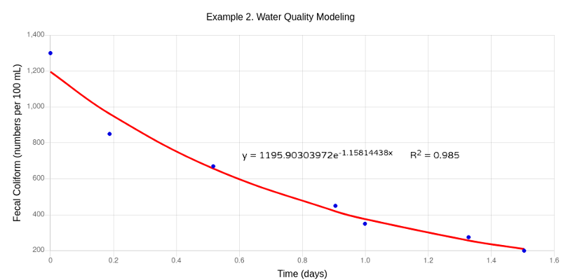
To solve the coliform die off rate, we will perform linear regression using Ordinary Least Squares (OLS) and the exponential transformation y = aebx. Results of the analysis indicate that a die off rate is 1.158 (day-1) would be a reasonable value at the water temperature on the day the samples were collected.

| River Station (miles) | Fecal Coliform (#/100 mL) |
|---|---|
| 12.8 | 1300 |
| 11.2 | 850 |
| 8.4 | 670 |
| 5.1 | 450 |
| 4.3 | 350 |
| 1.5 | 275 |
| 0.0 | 200 |
| Time (days) | Fecal Coliform (#/100 mL) |
|---|---|
| 0.0000 | 1300 |
| 0.1880 | 850 |
| 0.5171 | 670 |
| 0.9049 | 450 |
| 0.9989 | 350 |
| 1.3280 | 275 |
| 1.5043 | 200 |
Being wise engineer, you realize that most water quality models are temperature dependant and require input for reaction rates be expressed at 20oC. Models then will use a temperature correction factor, Θ, to adjust reaction rates based on the water temperature being modeled. A typical Θ value of 1.047 is used for coliform. The expression used to adjust for temperature is:
Kt = K20Θ(T-20)
Where:
Kt = first order reaction rate at water temperature T
K20 = first order reaction rate at 20oC
Θ = temperature correction factor (1.047)
T = water temperature, oC
We already solved the first order reaction rate (Kt) of 1.158 (day-1) at 24oC by regression techniques. Solving for K20 in the above equation results in 1.038 day-1, which would be the value to use in a water quality model. We will leave it as the obligatory exercise to the reader to solve for K20.
Your firm won the Request for Proposals (RFP) to provide engineering services for a local municipality to evaluate an aging wastewater treatment plant and make recommendations. After the evaluation was completed, an engineering report was prepared for various treatment alternatives. The most cost effective and thus recommended alternative was to rehabilitate the existing treatment plant. The engineer's estimate of the probable cost was $7,525,000 (2020 dollars).
In order to advance the project, a sequence of events must occur, such as adoption by municipal voters or board members to proceed with the project, regulatory approval of the engineering report, environmental impact statement, apply for government grants and loans, prepare detailed engineering plans and specifications, regulatory approval of the engineering plans and specifications, municipal bond resolution, put the project out for bid. The engineering report included a timeline for the project schedule with construction starting in the year 2024.
Being a wise engineer, you also provided the estimated project cost in 2024 dollars to be used in applying for government loans and grants to ensure so the municipality has the necessary funds to construct the project.
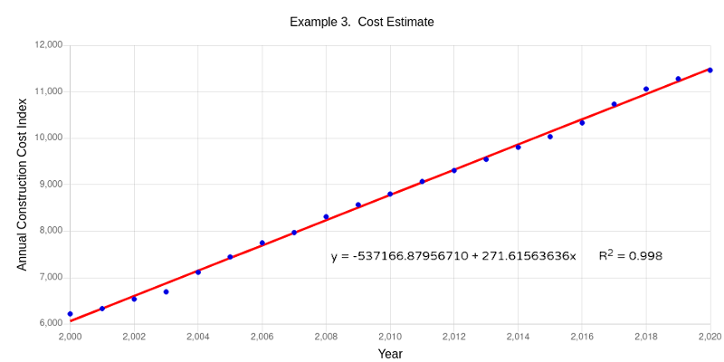
In order to estimate 2024 cost, you performed linear regression using the method of Ordinary Least Squares (OLS) based on Engineering News Record™ (ENR) Annual Construction Cost Index™ (CCI) from the years 2000 – 2020.
The regression analysis results in the equation Y = -537166.9 + 271.6156X. The coefficient of determination (R2) was 0.998, indicating a very good fit. Solving the equation for the year 2024, the estimated index value is -537166.9 + 271.6156(2025) = 12854.69. Using the ratio of the 2024 and 2020 index values, the estimated 2024 project cost is (12854.69/11465.80)*($7,525,000) = $8,437,000.
Without accounting for the additional $912,000 in the project planning, an unexpected financial burden could have been placed on the community and additional funding would be needed.

| Year | Annual CCI |
|---|---|
| 2000 | 6221.00 |
| 2001 | 6334.00 |
| 2002 | 6538.00 |
| 2003 | 6694.64 |
| 2004 | 7114.89 |
| 2005 | 7445.98 |
| 2006 | 7749.37 |
| 2007 | 7970.52 |
| 2008 | 8311.14 |
| 2009 | 8570.13 |
| 2010 | 8800.66 |
| 2011 | 9069.82 |
| 2012 | 9307.66 |
| 2013 | 9546.66 |
| 2014 | 9806.52 |
| 2015 | 10034.23 |
| 2016 | 10331.43 |
| 2017 | 10735.84 |
| 2018 | 11061.85 |
| 2019 | 11281.40 |
| 2020 | 11465.80 |